How to draw a Bode diagram (first-order delay system)

・ In Japanese
premise knowledge
・ complex plane

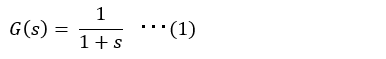
Explain how to draw a Bode diagram of the transfer function of a first-order delay system. (Reference: Basics of how to draw a Bode diagram)

■Transfer function of first-order delay system

as below.


Substitute s=jω into equation (1) and transform it as follows.

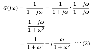
■Expressing the transfer function of a first-order delay system on the complex plane

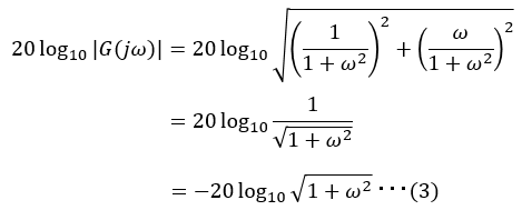
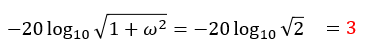
Express equation (2) on the complex plane as follows. A Bode diagram can be drawn by calculating the absolute value and angle of G(jω).

■Gain characteristics of transfer function of first-order delay system

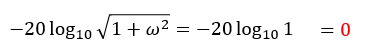
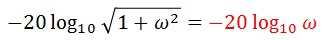
The gain characteristics are calculated in decibels, so they are as follows.



The characteristics of the above formula change depending on the value of ω, so we will divide it into cases.

■When ω<<1 (sufficiently smaller than 1)
From equation (3),


■When ω=1


■When ω>>1 (sufficiently larger than 1)



＜bode plot＞
From the above, the Bode diagram is as follows. The frequency at which the gain is -3dB is called the cutoff frequency.

■Phase characteristics of transfer function of first-order delay system

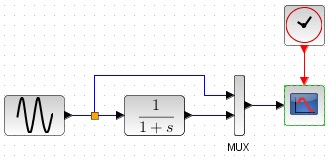
Phase characteristics are easier to understand if you think about them on the complex plane. This characteristic also changes depending on the value of ω, so we will divide it into cases.

■When ω<<1 (sufficiently smaller than 1)
Since the imaginary component is 0 and it is on the real axis, the phase is 0°.



■When ω=1
Since the real and imaginary values are the same, the angle to the real axis is 45°. The phase will be delayed by 45°.



■When ω<<1 (sufficiently smaller than 1)
The larger ω becomes, the closer it becomes to the imaginary axis, and it eventually converges to 90°.




＜bode plot＞
Based on the above, the Bode diagram is as follows.

■Check the characteristics of the first-order delay system by simulation

The results when ω=1[rad/s] are shown below. The black line is the input, and the green line is the output. (Reference: How to use scilab)

List of related articles TOP MENU Control theory Transfer function Transfer function Transfer function synthesis Closed/Open-loop transfer function Analog filter Low Pass Filter ・First-order delay system 　・Transfer function 　・Bode plot ・secondary delay system 　・Bode plot ・Butterworth filter ・Bessel filter All pass filter 　・Transfer function 　・Pade approximation Notch filter Band pass filter