Gain setting using the pole placement method
(PID control + a second-order delay system)

　・In Japanese
Premise knowledge
　・2nd order delay system
　・PID controll
　・Pole placement method
　・Transfer function composition

This section explains how to set the gain using the pole placement method when performing PID control on a second-order delay system.

■Transfer function of second-order delay system + PID control

The closed loop transfer function above is: (Reference: Transfer function composition).


here,



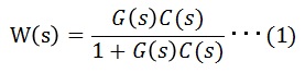
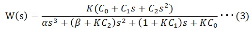
From the above, equation (1) becomes the following. (Reference: calculation process)

■Characteristic equation

The stability of the system can be determined by the value of the solution to the characteristic equation (2), so first calculate the solution to the characteristic equation. Here we use the idea of a reference model.

＜reference model＞
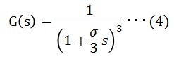
Assume the following transfer function.



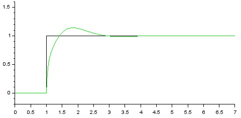
The solution (pole) s of this characteristic equation is as follows, so if σ is a positive value, it is stable, and if the value of σ is small, the convergence speed increases.

　
If you can express the solution of the characteristic equation in equation (3) in the same form as equation (4), you can set parameters that are stable and have a fast convergence speed. A transfer function that serves as a model like this is called a reference model. Now, I will explain the specific method.

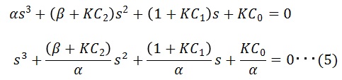
The characteristic equation of (3) is as follows.



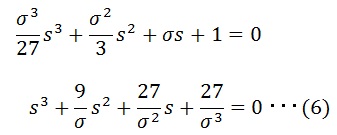
The characteristic equation of (4) is as follows.



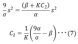
From equations (5) and (6),



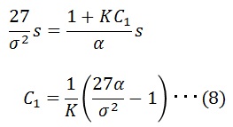
Also,


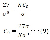
Also,


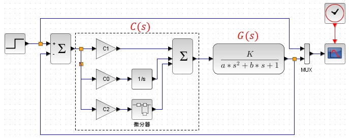
Now, by substituting equations (7), (8), and (9) into equation (2) and tuning σ, it is possible to set the desired gain.

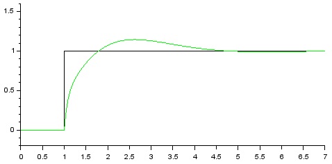
■Second-order delay system + PID control operation

The Scilab model is as follows. (Reference: Differentiator contents, Differentiator explanation)



■Parameter settings
It is assumed that the characteristics of the controlled object are determined in advance and are as follows.

　α=5,　β=10,　K=1

Simulate σ with tuning elements as 1 and 0.5. It can be seen that convergence improves when σ is made smaller.

＜σ=1＞


＜σ=0.5＞

List of related articles TOP MENU classic control PID Gain tuning Ultimate sensitivity method Step response method Pole placement method 　・2nd order delay + PID Application Filtered derivative Velocity-type PID PI-D type control I-PD type control Internal Model Control